NZ Rail Maps: Using Gimp To Georeference Retrolens Aerial Photos [7]: Extracting Mosaic Tiles

So I have been trialling the alternative overlay method with more files and have decided to redo all the mosaics for Auckland so far. This is a few days' work but as there are already some issues with accuracy in some of the more hilly areas or where the embankment is raised, it is going to bring improvements. However, file size savings are harder to nail down, and in general I think I am not seeing consistent meaningful reductions across a range of files. What I have arrived at to maximise file size saving, is to do a bulk crop to 50% of the original size, and then custom crop each layer to just the amount that is needed, that will vary from layer to layer depending on what is needed to align with the surrounding terrain (roads etc) to get smaller still. Currently this technique is being used on a big mosaic project, Auckland-Westfield NIMT, which covers 14 km of corridor and has around 180 layers. OK so there I broke my rule, by cropping the historical layers so much we can save a lot on disk usage and have more of them, but I am still having to test the water with so many layers in this project using just a small part of a very large canvas of 35 gigapixels which is probably the biggest canvas ever, as well, and that aggressive cropping is necessary to ensure the file size doesn't balloon unmanageably. Here's a screenshot of the canvas, with all the base tiles in place. The Port of Auckland can be seen upper left. This corridor was opened in 1930, the original route of the NIMT being the western line that became the North Auckland Line and Newmarket Branch dating from 1873.

This post outlines the last stage in this georeferencing process, which is to extract tiles from the mosaic project that can be imported into the GIS and used to produce historical maps that are accurate in positioning of features compared to present day maps. This being, of course, the major point of the whole exercise. There are some important considerations, the first being whether to use the same tile size, 4800x7200 in this case, as the base imagery, or combine a number of tile spaces into a larger sized tile. I tend to go for this latter option since it is just less work in extraction. The important issue here is to use the grid to get the top left corner to be the same as an existing background tile so that I can copy the coordinates from that existing tile when I need to make the sidecar files for the mosaic tiles. Sometimes there isn't one available and we will need to calculate the coordinates off the nearest available tile and here using EPSG:3857 with its coordinates expressed in metres we get a distinct advantage over a CRS that has its coordinates expressed in degrees because all you have to do, knowing the pixel resolution in metres, is make a simple calculation. In this case with this layer, at 0.1 metre pixel resolution of the base tile, each of those tiles covers an area that is 480 metres wide and 720 metres high. It then is straighforward to alter the top/left coordinates in the world file using these numbers.

The second consideration is how to name the new tiles. I always base my names on the original base tiles with a prefix. If the base tile gets scaled up or down, I also put a suffix on the original name to show that it has been resized. Let's say I have a base tile 93Y35-92S5Z that has been scaled double in each direction, I will have renamed it 93Y35x2-92S5Zx2. Then the prefix will be a single letter representing the station and followed by four digits representing the year. Then with a tile area that covers multiple original tiles I am going to use a filename that shows the first tile and the last tile in the range covered. So here is what my large mosaic tile's filename might look like: 

X1984-93Y35x2-92S5Zx2+93Y3Bx2-92S63x2.jpg

So in there we have station X in 1984, and then the range using layers that have been scaled up by 2 a side. Note the use of the + character which may not be permitted in Windows, this file name is legal in Linux which I use and which has far fewer filename letter restrictions than Windows. This is just an example - I don't know if I can cover all that large area in one file, as Gimp does have an export size limit, it may not be an efficient space to cover in one single file, and in this example we are actually not scaling 0.1 metre tiles up by two times anyway. 

My sidecar files are .jgw, .xml and .jpg.aux.xml and they all have to be given the same base name with the correct extension and we just copy the ones from the original base tile for the top left corner (93Y35-92S5Z in this example). The only change we need to make is in the jgw file - if we have scaled then the pixel resolution measurements need to be changed e.g. from 0.3 to 0.15 m. This is well described in previous posts. I described earlier in this post how I might change the top-left coordinates in the same file if I didn't have a set of sidecar files already downloaded to match the top left base tile in the area I am covering. Other posts on this blog describe the world file format in general and what those six numbers mean.

So hopefully in this series of posts I have adequately covered how to georeference the historical aerial layers in Gimp and how to get them into the GIS. Along the way I have learned some stuff as well, which is why I like to write these articles.

NZ Rail Maps: Using Gimp To Georeference Retrolens Aerial Photos [6]: Alternate Overlaying Technique

Today I am going to look at an alternative way of stitching together the source layers. I have to do a set of mosaics for the station of Kamo, which is the northernmost part of Whangarei. From a rail perspective there were two stations there. Just a little south of Kamo there was a coal mine which appears to have had a siding going off on the west side of the line, and although I don't know any more than that, I will include the NZR aerial images from Kamo right down to this area, since they are for continuous corridor. The idea that I am working on today is to reduce the amount of overlap between aerial layers. With every other project to date I skipped every second layer in the sequence but still found there was a lot of overlap between layers, enough to create various challenges I mentioned with overlapping, but not enough to be able to skip to every third layer. I want to look at reducing those overlaps, the potential benefits being a lot faster to overlay them in sequence, smaller file sizes and more accurate representation of the ground below with reduced perspective distortion. The way I did it before with every second layer was still overlapping quite a percentage of each layer and it being overlapped at one side, which means one side of the image will be more distorted.

In the layer sequence for Kamo down to the colliery siding the images are Survey 2788, Run A 1 to 3 and 2788 B 1 to 8. A total of 11 source layers. But I am going to use only the middle of each one of those. In addition because there is overlap between the A run and the B run, as is fairly common when the same rail corridor is covered by more than one run, because it goes around a curve and goes out of the side of the straight line of the existing run, I might be able to drop one or two layers. So what we need to do is to run Gimp with no projects open and open the source layers up using the Open as Layer command. Gimp creates a new canvas the size of the first layer and loads all the layers into it, centering them within that canvas. As all the source images are more or less the same size, they all line up with each other more or less exactly, or at least good enough for this exercise.

The obvious approach is to select a percentage of all of the source layers and apply that percentage to all of them. Using the centremost part of each layer is a good rule of thumb but you will have to check if this works with the source images you are using. But because you are using all of them, there is so much overlap everywhere that it's highly likely it will. The way to do this with Gimp is to use the Guides that you can set up from the Image menu. First of all, go to the View menu and select Show Guides. Then go to the Image menu and come down to the Guides submenu and if there are any existing guides visible and you don't know what they are then Remove All Guides. Then on the same submenu, New Guide (by percent). In the dialog select vertical or horizontal (you need guides that are at right angles to the rail corridor, but I set up both orientations to cater for both possibilities). Start with two guides at 33.33% and 66.66%.  The next step is to go through the layers one at a time and look at where the guides fall on them for example from A 1 to A 2 and see if there is enough overlap. In my case I decided to go for the middle 40% and therefore I went back, removed the guides and set them to 30% and 70% then there was enough overlap.

The next stage is to crop the layers and save them to be imported into the mosaic project. First thing to do is to create a selection that covers that middle 40%, which I do firstly by going to the View menu and turning on Snap to Guides, then I create a rectangle selection and use the guides to get the long edges into the right place. The short edges go up to the border, which we need to trim off in any case. This is why I didn't mention cropping the frame off each source layer as I did when I imported the full size layers directly into Gimp as I mentioned in a previous post. The way I am going to draw this selection is that it is a rectangle where the short edges parallel the rail corridor and the long edges are at right angles. This is how I get only the middle 40% of the rail corridor on each layer.

There are a couple of techniques for cropping in Gimp, just as a by-and-by, with different results in terms of their impact on the source layers. The obvious one to use is the Crop to Selection option on the Image menu. This will take the canvas down to the size of the selection and at the same time it will crop every layer to fit that canvas. As it happens this is the right thing to do with this project. The alternative which is useful to know if you want to keep the source layers at their full size, is to choose the option on the Image menu to Fit Canvas to Selection. That doesn't have an application to this particular project at all, but there are times when it's useful to have the full size layer available even if part of it is outside the visible canvas area and I just mention that in passing in case one day that is the situation you have, and there have been times I have used this alternative, for example when selecting a few layers from off a bigger canvas and saving them in a small canvas. Gimp will save layers that are outside the visible canvas, obviously using up more disk space than if all the layers are cropped within the canvas. Keeping the canvas just to the size you need is important because I discovered a bug in Gimp with a large canvas with only one small corner occupied that it will crash when saving. So my rule of thumb is only create the canvas size you will use and expand it as needed.

So use this Crop Image to Selection option to crop down all the layers at once. Then save to a new Gimp project file. I have 11 layers (A 1 to 3 and B 1 to 8), and the new project file has saved all of the middle 40% of 11 layers at less than 1 GB total, which looks really good so far. Now I am going to import additional base layers and my 11 segments of overlays into my mosaic project. In this case my base layers go from 93Y35-92S5Z to 93Y3B-92S63, which is a total of six columns (Y35-36-37-38-39-3B) and five rows (S5Z-60-61-62-63), so the first task is to increase canvas size by adding 36000 pixels to the top, the canvas being already wide enough for the six columns. My new canvas will therefore be 151200 x 52800 pixels since I added an extra blank row to ensure a one-row gap in the canvas between this geographical area and the one appearing on the canvas below, as I have multiple areas (different railway stations) shown on the same canvas. One thing when I started doing large projects is it doesn't matter how much of the canvas is actually used. What uses the disk space is each layer, regardless of where it sits in the canvas. I have had some very large canvases that only have an L shaped area along two sides occupied, maybe only 15-20% of the entire canvas, and there are no issues like wasting disk space because Gimp only saves the actual layers, not the canvas itself. It just saves the measurements of the canvas and the position of each layer, not every single pixel of the canvas itself. 

After resizing the canvas, use Open as Layers to bring in the base layers, being sure to first select in the Layer list the layer that you want the new layers to be inserted above, and if you want the new layers to appear in the right order then in the file dialog box select a sort order that is the reverse of the one you want. Then once the base layers have been imported and positioned in the right places in the canvas, bring in the overlays. You do this using the Open as Layers command again, but instead of selecting image files to bring in as one layer each, you select your project file that you created from cropping the overlays.  Gimp brings in all the layers from that project file into your current project individually, inserting them above the current position in the layer list in the same order as you had them in their project file.

Then you can overlay them the same as usual. That turned out for me to be a lot easier working with smaller layers, and the result was they came together in the mosaic project quite rapidly. I did change the layer order in one place, putting layer A 3 above A 2, and was able to dispense with layer B  1 because B 2 had enough overlap onto A 3, and I also found I didn't need layer B 8, so that got me down to 9 layers out of the 11 I thought I would originally need. After putting in the first layer, I can speed up the subsequent layers by just dragging them into the same size as each previous one and then do the underlap straight away, then line up the bottom edge. Even with the potential challenges of surrounding hilly terrain not lining up and significant changes in the general area - there is now a lot of residential development on the east side of the railway at the first Kamo station it was very straightforward. (Kamo had two stations both of them named Kamo, the earlier one being further south than the later one, and as both were open at the same time, the more northern one was originally named Ruatangata or Ruatangata Springs.) The amount of overlap (and therefore underlap) is much less and the narrower layer segments, for various reasons, are simply a lot easier to work with - because they are a closer representation of the actual terrain. I believe the result has fewer overlapping errors and is a more accurate representation of what is on the ground overall but this will have to be tested out in practice, and that is much more likely to be tested in mosaics covering large rail yards than with a station with a few tracks or a single track main. It's hard to work out any possible improvement in file size but as an exercise I went back to my original project, removed every second layer and the redundant layers and then saved it, the result was a file 50% larger than the original. When I saved my mosaic project in Gimp, it already had the full size versions of all the layers in Run A and Run B imported in, so it's hard to pick up the actual saving in disk space that might have resulted. I've taken out 17 full size layers and replaced them with 9 that are less than half the original size, but in their place I imported another 16 base layers. But anyway the new version of the mosaic project file is about half a gigabyte smaller than the previous version. So the whole I think there are going to be some physical benefits in resource usage as well.

So the net result of this exercise is that is how I will be doing my mosaics in future. Taking the middle 40% slice out of consecutive layers because it works out better all round. The overlaying process at this point can be described as:

1. Align and size an overlay along the long edges of the previous overlay (does not apply to first overlay)
2. Find the underlap point with the previous overlay (overlap of background for first overlay) and roughly align to it.
3. Line up the bottom edge to roughly the right place
4. Do Step 2 again more precisely
5. Do Step 3 again more precisely
6. Transform.

There is one more part to write and that is how to extract the mosaic tiles for the GIS. That will be Part 7 next time.

NZ Rail Maps: Using Gimp To Georeference Retrolens Aerial Photos [5]: Overlaying Multiple Layers

So in my last post I showed how to get started in georeferencing with the first overlay. In that post I put the second layer in to show how it would join onto the first layer. The aim of this part is to show how to add additional overlays and how to deal with the overlap between one layer and the next. 

Right now from the last post this is what I can see on my computer screen of the Whangarei rail yards and sidings. Whangarei has a main station yard and a separate port area with its own sidings. The port used to handle container traffic until it was all moved to Marsden Point (which is near the heads of the Whangarei Harbour, whereas Whangarei is at the top) around 20 years ago. There has been huge debate ever since over the lack of a rail link to that port, and the rail-friendly Clark Government started the process to build the spur line that would come off the North Auckland Line at Oakleigh, only 14 km south of Whangarei. But then there was an election and the anti-rail Key administration came into power and stopped all the rail work. It is now being resumed by the Ardern government and probably the construction will be approved to start in the next 12 months. Anyway those port sidings are still in place to some extent and some ships still come into the port so the maps of Whangarei will document that but we need seven overlays in the D series and two in the F series, a total of nine. I am also mapping Kamo which is to the north of Whangarei as the same series of aerial photos Survey 2788 has two runs that cover that part of the Whangarei urban area and the Northland 0.1 metre urban area aerials are also available for there. 

But for now let's have a look at overlaying D 5 onto D 3. As you can see I am not getting across much distance with each overlay. I can do a rough measurement from the grid because I know there are 4800 pixels wide and 7200 pixels high and each pixel measures 0.1 metres on a side, so with the two overlays so far covering roughly 2 high and 2 wide, so far we have covered an area 960 metres by 1440 metres, or 0.96 km by 1.44 km. It's easy from that to understand how the disk space gets gobbled up because I have to be able to work at this high resolution to get the detail visible down on the ground that I need and that means a lot of layers. This particular project file covers Oakleigh, Portland, Whangarei, Kamo and possibly Hikurangi / Waro in one canvas which is not continuous but broken into separate areas for each station, and it's currently on a 52800x108000 canvas with 69 layers and is taking up 10 GB on the disk. As I mentioned previously my rules are not to exceed 100 layers and 20 GB disk size although I do have a small number of projects that are around 30 GB but Gimp doesn't seem to be able to handle much larger than this without crashing a lot. But when covering a long urban corridor and having to split it across multiple files, then an extra complexity is to deal with the overlaps between the edges of each file. Of which more later.

One of the reasons progress is slow is that even with skipping to every second image in the NZR survey, there is still up to 50% of each image overlapped and that is a lot as you can understand. It lends weight to the idea of taking all the images in the survey and just chopping the middle out of them. That is something I might try with Kamo because I could save a lot of disk space that way because the overlapped pixels are just wasted duplication that uses up storage.

So now in Gimp I've selected D 5, put it into unified transform, and started lining the top of it up with the bottom of D 3. Now, it pays to be smart about the order in which Gimp draws layers, because there is this overlap in the case of these overlays. The base aerial photos are all nicely broken up into tiles that don't overlap, they all just nicely fit against each other in the grid, but we don't have that convenience with the overlays. So if I have three layers in the layer list the highest up one will be drawn over the top of the ones lower down in the list. And that calls for some careful thinking when doing the unified transform, because what you see in the preview is the overlay that is selected for the transform, drawn over the top of all the other layers and contradicting the order in which it will actually be drawn when the transform is completed. Here's a screenshot that illustrates that pretty neatly.

So what you can see happening in this screenshot is I've done the first stage of overlay transform. I've put the pivot right up the top of D 5 at a point that I am confident I can line up on that is also present in D 3, and then I've gone down to the bottom of D 5 and dragged a size handle to size the overlay to match the surrounding terrain pretty well. So we start by overlapping somewhere near the top of our current overlay, because that is the easiest until we get the overlay to the right size. Then once we have that sorted, we now have to "underlap" as I call it. We have to align the overlay at the bottom of D 3 because that part of D 3 will be drawn over the top of D 5 all the way to the bottom edge of D 3. You can see where the overlay transform's frame is, the handles and the pivot at the top of the frame. But down near the bottom of this screenshot, what's underneath changes to colour instead of black and white. That's where the bottom edge of D 3 actually reaches to and that's where it is most critical to actually line up D 5 because that is where the join between the two layers will actually be drawn. 

When you come to do overlays on rail tracks, these old aerial images have marks that were specially placed on the ground by NZR staff. They would paint a sleeper completely white over its whole top and then add white paint on the centre sections of the sleepers on either side. The frog rails and guard rails on turnouts are usually also painted white, but this is more to highlight them as a safety hazard when crossing over the rails in the yard, as someone could get their shoe stuck in the gap. This is what the result looked like. The purpose of this was to make it possible to overlay the aerial photos into a mosaic that was printed out on a big piece of paper that was used by the engineering staff. I have seen these big printed plans which were over a metre by a metre when printed out and some of them are in storage in archives around the country.

It is a bit harder to get the join between two layers exactly right when it isn't actually on one of the overlay edges, partly because you have to take the preview opacity up and down to check the fit, and because the overlay at 100% opacity will not show the join at all, it will look like the join is at the top of D 5 instead of at the bottom of D 3. Before Gimp was updated to 2.10.18 with the Readjust feature, it was a lot harder to do a proper alignment at these joins and one trick I used was to do the overlays starting from the bottom of the Gimp layer list instead of the top because the preview would be correct for the layer order, another trick was to reorder the layers in the layer list if the join ended up being rough. But especially since Readjust became available it is now much easier to do these joins really smoothly and that has made a big difference to this task.

So now I am going to move the pivot down to the bottom of D3 and line things up down there. At this stage I still have the transform frame at the full size of the overlay and haven't used Readjust, which moves the frame and changes its size. By bringing the preview opacity up and down and finding the exact point of overlap, I can get a very smooth join. Here the shortcut keys I have set up to step opacity up and down 10% per step are very useful to preview what the join will look like. Basically you are comparing the overlay at 100% to the overlay at 0% and looking at how smoothly it overlaps close to the join. You can get a pretty good feel for how that join will look and in the case of a rail yard or some other situation where the join is wider than a track or two, you want to be checking all the way across. Bring the pivot down to that join, put it on some key feature like a main line, and if necessary use the Readjust to change the size of the overlay at the join so you can get it looking really smooth. Just remember Readjust moves the pivot to the centre of the new transform frame, and that you can only ever reposition the overlay by dragging inside the transform frame regardless of its size.

Once you have that pivot in place and have the join looking good you need to check at the edges of the overlay again for the underlying base imagery you are lining up on, if necessary using Readjust to make a really good smooth alignment, again being aware with Gimp 2.10.18 you need to move the pivot back to the join when you press the Readjust button, then finalise by checking the join is still correct, and then we are ready to transform. In this case the most important alignment for the bottom of the overlay is the main rail line heading south, and for the sides, it is the surrounding streets and houses, because with no clear features near the bottom to ensure we have the bottom of the overlay in the right place, we have to use features out to the sides to help check our alignment. Here's the result as we have it now, with a really smooth join that I am not going to zoom in but I got it really neat again across the rail yard, but with varying results further out, as we'd expect.

And so I will carry on with the rest of the overlays to get all the way down, all nine of them.

There is one more thing to mention and that is when you are doing a continous corridor, like in an urban area. In reality, NZR had corridor surveys of various types done, with the major main line corridors completely covered, but it's impractical for me to do that myself and use all those aerial photos. So typically in rural areas I am just doing a few stations by themselves, but in the major urban areas, such as the five main centres, continuous corridor is what I do. Now it's inevitable that I will hit the layer or file size limits that I work to and such a segment of corridor will end up being split over more than one file. For example earlier on I did a continuous corridor from Newmarket to Waitakere in Auckland which is a total of 36 km that ended up going across three files in total. When you get to the edge of the current file what you do is copy the overlay that is at the edge and the underlying base layers to a new file. There are a few ways of doing this such as creating a layer group, putting the overlay and base layers relevant into it and then dragging it to a new canvas and then saving that to a new file. Another is to crop the original image down to the base layers that cover the area occupied by the edge overlay and then save to a copy of the original file. The reason for base layers being saved with the overlay is in the new file you can drag all the layers together (including the overlay) by using the layer linking in Gimp's layer list, into the grid in the new file so that the base layers are lined up properly in that grid, and then add the rest of the base layers and overlays as required to the file. This ensures you don't have to realign the overlay and also that the overlay is still exactly in the same position as it was in the original file, so that new overlays you add to the new file can be aligned to it and therefore the extracted tiles will line up perfectly in the GIS.

Part 6 is going to look at how to extract tiles for a GIS from the Gimp mosaic projects I have been creating, because that is the ultimate aim of this process.

NZ Rail Maps: Using Gimp To Georeference Retrolens Aerial Photos [4]: Getting Started With Overlaying

So now we can look at how we actually do the georeferencing. This happens as a multi part process, and explaining the steps gives you an understanding of how it all works.

The basic of georeferencing a historic aerial photo, is that by aligning it to a current aerial photo, of which we know the area that it covers, we can make the historic photo cover the same area as that current aerial photo. So this makes it easy to trace or otherwise reference features from the historic aerial photo and see a comparison with the current aerial photo. In NZ Rail Maps I use the historic photos to trace, for example, old closed branch lines, bypassed sections, and old yards and buildings at stations. This gives me a documentary record of historical features of a rail corridor and these features are displayed on the resulting map.

We do the georeferencing by using Gimp's transform tools to overlay the historical image over the top of the current image, or a grid of images (tiles), that cover the same area as the historical image. In practice we usually have multiple historic images in each Gimp project file, that cover multiple stations or yards, or a continuous length of corridor (most commonly in an urban area, where there can be lots of points of interest between stations, such as sidings). For example, in the five main centres, I have created Gimp projects that cover continuous corridors for a section each. The Auckland corridors are at present up to 10 km in each Gimp project each because they only have one historic layer. Christchurch corridors created so far are only a few km each because they have multiple historic layers from different eras. It doesn't take much distance working with originals of resolution 0.075 metres and NZR survey images of 1:4350 scale to start adding up to gigabytes of disk space in a Gimp project, when just one 4800x7200 background tile has 34 million pixels in it.

The overlaying is the tricky and slow part. We have to try to make as many features on both the current background image and the historical overlay image line up as we possibly can. For a variety of reasons this can be difficult. The major one is perspective distortion. When a photo is taken, with any type of camera, the subject is most accurately rendered where it is directly aligned to the centre of the camera's lens. At any other point of the image, the camera is effectively looking at that part of the subject from the side, and the resulting distortion gets worse the further you go out to the side of the lens. On a typical photo taken on the ground, there isn't really an issue with that. But when the image is taken for the purposes that an aerial photo is taken for, where we want to get an accurate representation of what is on the ground below, and given the distances incorporated in each photo, the distortion makes that difficult. That's a key reason why adjacent photos in a survey run are given a big overlap. You could get a really accurate aerial view by taking the centre most piece of each photo and joining it to the centre most piece of the next photo which would be easy with the amount of overlap on, for example, the NZR station surveys. I could actually do this, but so far, I have just used every second image. Because of the distortion, overlapping features that go above the ground like buildings are difficult. So are features that are on hillsides. The most challenging ones from a rail perspective are where a railway line on a raised embankment runs next to tracks that are on the flat, such as in the Dunedin railway yard where the main line is raised, and the technique for that is to have two copies of the historical image, one for the raised and one for the flat area, overlay each one just for the raised or flat features, and then overlap them using masking.

OK let's get started. Typically the layer list will show your Retrolens aerial photos at the top of the list, and the base imagery from Linz down the bottom of the list. So that your historic aerial photos are always drawn on top of the base images. Here is a typical Retrolens image that you've downloaded and imported into Gimp. First thing is to rectangle select it, and crop off the edges (shown here with the rectangle selection in place). 

Using Layer menu, Crop to Selection. Repeat this for every layer in the stack that is the same size. Change the selection rectangle if you have layers that are different sizes or have different borders. The borders being of no use to us.

Next step is to do the overlaying, one layer at a time. First, check that Snap To Grid is turned off in the View menu. It gets annoying when you are trying to precisely position a layer and Gimp is snapping it to a side of the grid. Also, there will still be a selection active from the cropping stage. Go to the Select menu and choose None to make sure there is no current selection.

Back in the day, with earlier versions of Gimp, you would have to use different tools to perform the overlay task. When I started using Gimp, I used the Scale tool to size the overlay, which doesn't have any preview capability, so I would just try scaling by trial and error until I got the correct size. As you can imagine this was very time consuming. Next step after that would be the Rotate tool, to get everything to line up. After a few months I discovered the Unified Transform tool. This is a new feature in Gimp 2.10 and it combines the function of both these tools and it offers a full preview, which lets you do the lining up. We recommend to make things easier, set up the keyboard shortcuts mentioned in Part 3 to enable you to quickly change preview opacity, canvas rotation, and zoom level.

Select the Unified Transform tool in the toolbox. Then select the first layer in the layer list and click on it. Your layer will be displayed as a preview frame, with a pivot (a circle with crosshairs inside it) in the centre and various handles at the corners and along the sides. Familiarise yourself in the documentation about how to use these handles. Now click somewhere within the layer preview and drag it to somewhere over the base imagery. Look for a feature that is common to both layers. Then drag the pivot from the centre of the preview to the common point on it. My favourites for common alignments are the ends of bridges, or a set of points, but often I use road features as well. It only has to be approximate at this initial stage. Once you have the pivot in place on the preview frame, set the opacity to zero and drag the entire preview frame so that the pivot sits over the same place on the base imagery. Then increase the opacity and confirm the pivot is properly located.

One caveat that is important when doing a unified transform. If you press the wrong key on the keyboard, it may start the transform before you are ready. This is an annoying feature in the current version of Gimp. Many's the time I have pressed the wrong key on the keyboard and the transform starts before I am ready.

In the above photo, we have positioned the preview of 2788-D-1 over the appropriate place on the base imagery, with the pivot very near the top centre, lined up on the end of a railway bridge.

Once the pivot is in place then decrease the preview opacity to about 50% and use the most convenient resize or skew handles to drag the preview to fit the underlying base imagery. To make this work off the pivot, go to the Tool Options dock and ensure that under "From pivot" the Scale option is checked. This makes sure everything else scales centered around the pivot when you drag those handles. Then resize the preview and try lining some other features up in both images. Use the opacity adjustments to compare the preview and base as much as needed and adjust the preview position and size to suit.

Youll see there are stretching (square) handles at the corners of the preview as well as in the middle of each side. But what if you need to have one in another place closer to where you are working with the canvas zoomed right up and the nearest one is out of the view? This is where the Readjust feature comes in. Press that button and you'll get a new frame right where you are viewing at the moment, instead of one around the full preview. Just note that the pivot moves too, to the centre of the new frame, and most likely you'll want to drag it back to where it was before.

 Somewhere along the way you'll want to recheck the pivot position to make sure the preview is properly lined up there as well. If you need to adjust the preview position at the pivot, then check if you need to redrag a side or corner handle to resize the preview and line the rest of it up again. I usually try having the pivot as close as possible to the top of the preview, while I am resizing at the bottom-most side. For the Retrolens layer 2788-D-1 I initially chose to line up on the railway bridge over Walton St. The bridge has been lengthened since 1975, because the road it crosses has become a  roundabout, which makes it tricky to line up on. I really need to check against something else on the ground that it will line up. And because it's raised above the ground, the tracks lower down might not line up so well. After a lot of checking, I realised I needed to move my pivot to a different location, because the southern end of the bridge was just not the right place, because the bridge was extended at that end. But the north end of the bridge was not right, either. Eventually I decided the best option was to line up on the next bridge further north (Water St) which meant adding an extra base tile at the top of the canvas and increasing canvas height.

Once you are sure you have the preview lined up as best you can over the base image, check that interpolation is set to the right setting in the Tool Options dock (I use Cubic), then click the Transform button and away it goes. When the Transform has completed, the next thing that is important to do is to lock the position of the transformed historic layer, so that it can't be accidentally dragged out of place on the canvas, because unlike the base tiles, it isn't aligned to the grid in any way.

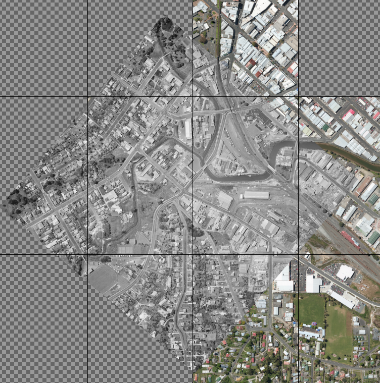
The finished result after overlaying the first historical tile for Whangarei railway station, which is Survey 2788, run D, photo 1, over the Linz 2014 0.1m base imagery for the area. The main railway yard is about half covered by this historical image. Meaning that the join onto the next historic layer, D 3, would be highly visible as it would be across multiple tracks. One way to avoid this would be to use a different layer to start with (like maybe D 2 instead of D 1) that would push the edge out, and another way is to exploit the overlap itself and use a bit of masking to move the join to a different part of the overlap.

In this case I went ahead with D 3 without any masking and managed to get a nearly perfect overlap, as you can see below. But there have been plenty of times when it hasn't been quite so smooth.

An overlap is going to be less than smooth when there are rail wagons or service buildings across it, for the reasons I mentioned near the top of this post. And sometimes, there is simply too much distortion to make it ever work. In this case, it looks perfect across the rail yards, but further out, across suburbs and houses, there are bits of buildings cut off and misaligned, as shown below.

 

In this case, because the rail yard ended up near perfect, I didn't bother checking the result further out. The reality, as I mentioned above, is that quite often it is impossible to get a perfect alignment all the way across an aerial photo. I could have worked on improving the alignment towards the edges and then the rail yard would have been misaligned.

 

Gimp has got better over time, with the readjust feature (a result of a feature request I made on the Gimp forum) making it much easier to get perfect alignments across joins. I'll look at the challenges of doing this in Part 5.

NZ Rail Maps: Using Gimp To Georeference Retrolens Aerial Photos [3]: Getting Imagery Into Gimp

So let's get this rolling. First thing I need is to download the layers from Linz Data Service. Which in this case is at the following URL: https://data.linz.govt.nz/layer/53399-northland-01m-urban-aerial-photos-2014-2015/

The layer is called Northland 0.1m Urban Aerial Photos (2014-2015) and covers the stations of Whangarei, Portland and Kamo. It also covers the port area of Whangarei, which is good, because the NZR station surveys cover all the extra bits. I chose to download the entire layer, which is 4.8 GB. I find it preferable to use a download manager when handling downloads of this size. Since I use the Firefox Developer Edition browser, the best download manager is uGet. Although a bit fiddly to set up, it works well, especially since I have my computer set up to save my profile whenever I need to reinstall the operating system.

I'll also note where I get the NZR survey images from. I'll go to the Retrolens site and zoom it in on the Whangarei rail yards. Just typing in "Whangarei" and zooming in on that word on the Retrolens interface is enough in this case, because it conveniently brings us right to the railway station. Often though this is not the case and you'll find Retrolens thinks the centre of an area is way out in the countryside in the case of smaller townships and localities. It pays basically to have a look at another map, find a street name close to the railway station, and put that into Retrolens to make it easier to find the exact part of the map that I want to look up the aerial photos for.

The NZR survey is No.2788, with six different runs, from A to F, covering all the way down from Kamo to the Whangarei Port, and all of it was captured in 1975 at a scale of 1:4325. If I start from the rail yard area, on the right hand side of the Retrolens web site, I can see the aerial photos for an area, and I'll be looking for the ones that have a date of 5/01/1975. Clicking on one of these (I only need one of them at the moment, and it doesn't matter which one) will come up with more details, at which time I can confirm the survey number SN2788, the run number and photo number (the run number is going to be between A and F in this case but it doesn't really matter that much) and the scale is 4325. This scale in particular, or 4350, is virtually a unique signature of the NZR station surveys that can help you to identify them on sight, but in case you are unsure, view the labels in the margin to see if it says "NZR" or "RAIL" anywhere. Some of the aerials I have downloaded around Auckland and Wellington of the rail yards there are an even larger scale than 4325 or 4350.

Now here's a couple of little tricks to download all the images I need from this survey. First of all I'll click the Large button and bring up this image in the Large size, which is the highest resolution I can download from Retrolens. Now in this case the URL of this image is as below (so you can save yourself a bit of work by just skipping the above steps and going straight to this web page: 

https://files.interpret.co.nz/Retrolens/Imagery/SN2788/Crown_2788_D_3/High.jpg

Now, the fact is all NZR surveys start at Run A and photo 1. So I could go through the Retrolens site to find every single one of the images and get them. Or I could just change the letter D in the above URL in the address bar on the browser to the letter A and the number 3 to the number 1 and then press enter with the new URL to get 2788 A 1. And that is exactly what I do. This is a much faster way of downloading all the images from Retrolens. And when I hit a 404 error at the end of run A, I can start with run B photo 1, knowing in this case they go up to run F.

The other trick is usually you won't need every image from the survey, because they overlap enough that in 99.9% of cases with an NZR station or corridor survey, there is so much overlap that you only need to use every second image. Generally, I download every image, and then decide which ones to import into Gimp, which may be A 1, A 3, etc but sometimes it can be A 2, A 4 etc. Obviously choosing to use all the images just makes a lot more work for you in Gimp, but it also is going to increase significantly the amount of data that is stored in the file and make it bigger than it needs to be. 

The amount of disk space I have used to create mosaics is such a challenge for me to manage that I am sooner or later going to have to implement an economising strategy of actually deleting project files, simply because I can recreate them quickly in future with the extracted mosaic tiles, at the cost of a small loss of quality. At the moment my computer has more than 1.5 TB of Gimp mosaic originals stored on it, and I have decided I am simply not going to upgrade it to 4 TB disks, so managing the use of the 2 TB disks is what I am actually doing in practice. The extracted mosaic tiles in Jpeg format use much less space than Gimp does. That's understandable because the Jpeg format is lossy one-way compression, whereas Gimp is using lossless two-way compression that can recover all of the original data. If Gimp had some way of saving an archive copy of a project so that it was lossy compressed that would save a lot of disk space, and since that isn't practicable, the alternative is to split the files into lossy extracted mosaic tiles, which save a lot of disk space, and delete the project files. So far I haven't deleted any project files but it's inevitable I will have to do this sooner or later.

Anyway back to the maps. So we want to lay out our background tiles downloaded from LDS in the Gimp canvas. First thing is to set up the Gimp grid to 4800 pixels wide x 7200 pixels high. Next thing is to view the grid, and then turn on Snap to Grid. Then with a blank canvas, or no canvas because it will create one if there is nothing open, use Open as Layers to load the layers JPEG files from LDS. If you want them to appear in the "correct" order in the layer list, set the filename sort order in the dialog to Filename descending, this is because of the order Gimp adds the filenames to the layer list. They will all be displayed stacked on top of each other in the middle of the canvas and each one will be a separate layer. 

Then you need to increase the size of the canvas, to a multiple of 4800 pixels width and a multiple of 7200 pixels high. Once you have that, then start dragging the tiles into their place in the grid. Select the first layer in the list (right at the top) and then drag them one at a time. This is where Snap to Grid comes in handy. The filenames are based on a column reference followed by a row reference. The filenames use the digits 0 to 9 in sequence, followed by capital letters, then increment the next column of digits and back to 0 again. E.g. 50, 59, 5B, 5Z, 60 etc. But Gimp's filename dialog gets this order wrong for some reason (at least in Linux it does). There are a small number of letters missing from filenames, notably the five vowels. The tiles are usually all 4800x7200 wide, which is why I set up the grid to these settings. It pays to download a bigger area than you actually need, because LDS has this nasty habit of serving you fractional tiles around the edges of your crop area, which can be tricky to work with.

Next step: load the Retrolens images using the same Open as Layers command. They will also be stacked in the middle of the canvas. You don't need to do anything with them just yet so don't drag them anywhere as the next step (which will be in the next post) is most conveniently done to all of them whilst they are still stacked together. Right now is probably a great time to save your Gimp project. Have a cup of tea or a coffee and then start reading Part 4 of this blog series. Here we'll actually prepare the images and start overlaying them.

NZ Rail Maps: Using Gimp To Georeference Retrolens Aerial Photos [2]: Preliminary Considerations

So I aim to write one post every day about this topic (this post was supposed to be finished last evening but has stretched through until this morning) until all the parts are completed, there are probably three or four parts. This is easy because I am doing georeferencing at the moment on a particular volume of the NZ Rail Maps project.

Firstly, the choice of GIS project CRS. This relates more particularly to the GIS and strictly speaking is not relevant to the georeferencing task but is worth considering if your GIS project intends to use the Linz WMTS layers at any stage.

When you are creating maps in the GIS you need to consider the CRS of the project and this is very important if you are using Linz's WMTS live aerial photo layers. I use these layers for tracing all the current features of the maps and have been doing so for only the past year. Prior to that, I downloaded the individual map tiles for every rail corridor from the LDS website, but now I only need to download what I actually use for georeferencing.

Linz only supplies its WMTS layers in two CRSs, which are EPSG:2193 (NZTM2000) and EPSG:3857 (WGS84). If your project is not in one of these CRSs, using WMTS is only possible if the GIS can transform the CRS on the fly, and this can be fraught with challenges. In my case, I selected EPSG:3857 for my maps some years ago because of its compatibility with Google Earth KML. Even though I no longer import KML files into my maps in order to ensure there will be no licensing challenges in the project, I have stayed with EPSG:3857 as the project CRS.

If your project is not able to use one of the available CRS that is supported directly by Linz WMTS then downloading all of the tiles you need to cover your corridors and importing them into the GIS to provide the contemporary base imagery for the area being mapped, if this is what you are using, is the alternative. You will need some of this imagery as the georeference base for Gimp in any case. The difference with using it in a GIS and using it in Gimp is that the GIS will be able to load JPEG or TIFF files directly without expanding them out of their compressed state. However, when you import the tiles into Gimp, it breaks everything into separate pixels without the benefit of JPEG compression, and as far as I can tell, the resulting file size does not have the same level of compression that is possible in JPEG. I am not totally sure of this, and I know Gimp has its own compression built in, but I have to be able to account for a small volume of tiles becoming a big volume of Gimp project data.

Secondly it is very important to ensure Gimp is configured with adequate tile cache as the transform tools for handling large images will use up a lot of swap space. My computer has 32 GB of system RAM and 168 GB of SSD based swap space that Gimp can use. At the OS level, the SSD is configured as a Linux swap partition, and then in Gimp, I set the tile cache to 200 GB and it uses the 32 GB of RAM and 168 GB of the swap partition (which in practice is larger than this to allow for other system or application use). As a rule of thumb you could expect to be able to handle a Gimp project with a filesize up to 30 GB with this amount of tile cache. My experience has been not to push larger file sizes (generally I go with no more than 100 layers in my projects as another rule of thumb) since Gimp is more likely to crash during a save operation resulting in data loss. I have also experimented with another computer that has just as much SSD swap available but only 8 GB of RAM and this computer is far less able to handle 20 GB or larger project files and will often crash trying to load them, even though it is nowhere near using up all the swap space. It seems that both the system RAM and SSD swap are important but the amount of RAM makes a bigger difference to performance and stability than the amount of swap.

Thirdly, when you are doing transforms in Gimp you'll want to consider the best interpolation algorithm. Interpolation is what happens when you increase or decrease the size of a graphical layer. This is because the existing pixels are either being increased or decreased in number, and information from the existing pixels has to be sampled to make the new pixels. If you do a scale that is a whole number multiple of the existing size then each pixel just gets cut into the appropriate number of pieces needed, for example scaling by 2x each size means each pixel becomes four new pixels. But in real life we work with all sorts of scale multipliers and this process becomes a lot more complex. The interpolation algorithms are designed for various capabilities and Gimp has a few different ones supplied. When I started doing this stuff I tried with the most intensive and therefore slowest interpolations, LoHalo and NoHalo, but after a while I found that using Cubic gave just as good a quality with a much faster transformation speed and that has been what I have used ever since. 

It's worth noting that I found the scaling process counter-intuitive until I worked it out in my head after a while. To go from a pixel size of 0.3 metres to 0.15 metres, you scale the layer up 200% each side. I had always thought you would shrink each pixel down to half its previous axis by scaling at 50%. However, what you are actually doing at that point is creating new pixels with 50% of the previous information in them and so actually losing resolution rather than increasing it. When you are scaling up 200%, you are doubling the number of pixels so that each pixel contains less information and this is doubling the resolution. You end up with a layer that contains four times as many pixels, but when you tell the GIS to draw them at half the original size, the layer occupies the same area of the screen as the original.

The key reason we want to scale 0.3 m to 0.15 m, or perhaps 0.4 m to 0.1 m, or 0.75 m to 0.15 m, is that we want to avoid downsampling our historical layers too much. I found this out early in the piece with one project having to use 0.3 m background, putting a 1:5500 corridor survey image onto it, scaling that down in the transform too much, and losing too much detail. So these considerations have been worked out by trial and error. I now decide that base imagery where the size of a pixel is more than 0.15 m is a bit too big. I am still working with a lot of 0.3 m base imagery around NZ and scaling it to 0.15 m is the best way to deal with it. The result is a larger tile size and it is easier just to go with those larger tiles than to try dividing up the new tile into four tiles of the original size, because they have to be given a new naming scheme, and because you have to work out the coordinates of the top left corner of something that is spaced halfway along one side of the original tile, which makes for extra work. I tried this for a while but eventually I came around to understanding that a bigger tile, that is actually drawn by the GIS at the same physical area as the original by telling it the pixels are half the original size, is not enough of a deal to warrant getting pedantic about the size of the new tiles.

There is one more thing to think about and that is the merits, if your station doesn't fit within one tile, of making the mosaic tiles that you import into the GIS, cover more than one of the original tiles footprint. This is just done for the sake of convenience reducing the number of files you have to copy or store. Each tile (JPEG is the format I use) apart from the graphical file which takes up megabytes on the disk, has three sidecar files, which each take at most a few kB. You are not really saving a lot of disk space by reducing the number of files, but if you are creating the sidecar files for your mosaic tiles by hand, you'll appreciate having a smaller number of steps (I wrote a script to copy the sidecars). The main downside is the GIS will take longer to refresh larger tile sizes. Gimp has some sort of limit to its export functionality or plugin that will limit the actual size of your exported tile. When you combine multiple tiles into one bigger one, you do have to create each new tile as a rectangle and look at how a bigger area can be divided into multiple pieces. You also have to know the top left corner coordinates of the new big tile and the easiest way to do that is to put the top left corner of the new tile in the same place as one of the background tiles you got from LDS. Well, I'll try to explain these little details more as we work through the practical steps.

One more thing is to make Gimp easy for you to use. For me, that is by setting up the right shortcut keys so that I can make things happen really quickly. The key ones for me are:

• Zoom level - this is on the View menu, "Zoom In" and "Zoom Out" in the keyboard shortcuts interface. I have these assigned to + and - on the numeric keypad, which just allows a single key to be used to zoom. I have also experimented with using the Ctrl key with the - and = keys on the main keyboard.
• Canvas rotation - this comes from the Flip and Rotate submenu on the View menu. In the keyboard shortcuts interface, within the View menu section, the actions that I find useful are "Rotate 15 degrees clockwise", "Rotate 15 degrees counter-clockwise" and "Reset Flip & Rotate". These are assigned to Ctrl+., Ctrl+, and Ctrl+/ in my case.
• Preview opacity - the transform tools we are going to use all have previews which we use to line up the overlays with, before pushing a button to carry out the actual transform. We have to be able to compare the background and historical images at various levels of opacity and it's convenient to be able to go quickly up or down the levels. This is found in the Tools section of the keyboard shortcuts interface where it is programmed with the actions "Tool's Opacity: Increase by 1" and "Tool's Opacity: Decrease By 1". In practice, the steps are actually 10%, which is actually quite satisfactory, and there are also actions for 10, which I would use if it hadn't turned out that the 1 action actually turns out to be 10. I set these to be the , and . keys. The reason for using these keys is they look like left and right arrows because they are the < and > keys when shifted.

So next time we will look at actually doing the steps with Gimp, based on a real situation, this is creating a historical mosaic for Whangarei that is being done right now for NZ Rail Maps. The blog post will be written alongside the actual steps that are being done to create the historical mosaic to cover this station. This is part of Volume 1 of NZ Rail Maps that is being updated at the present time. The next post will appear later today because the schedule is actually one post a day and this post is being finished half a day late but the schedule will be caught up.

NZ Rail Maps: Using Gimp To Georeference Retrolens Aerial Photos [1]: Introduction

OK so here is another post in the NZ Rail Maps category and this post will explain how I carry out the georeferencing of the historical Retrolens aerial photos to produce the maps for the NZ Rail Maps project. This is a very rewarding aspect of the project but it does take a lot of work to complete, and whilst it is my desire to have the maps produced for the majority of stations in NZ being documented historically, it may not be practical to achieve this for more than a few hundred locations in practice.

This is the first of several posts that will outline the various steps needed for this particular process and this particular post introduces the process,

The first question to be resolved is whether to use this system at all. There have been in QGIS software and possibly other GIS packages, tools or plugins provided that enable georeferencing directly within the GIS. The plugin for QGIS is poorly designed in my view and I had considerable difficulty in making it work. It is not fully visual in that it is not possible to preview the final result, so it does have limitations. I had previously experimented with the image overlay capability in Google Earth but found that it was limited in its design.

So using Gimp has been arrived at over a period of time, due to its being best supported. The main downside of using Gimp is the large files that are generated by it. These vary, but for example to cover about 10 km of track distance with one generation of historical aerial imagery can result in about a 20 GB disk file in order to get a desirable resolution for picking up all the details needed for trackwork. This has largely been arrived at due to the source resolutions available. NZR had their own surveys done for major stations and also major corridors, and these have scales varying from  1:3000 up to 1:5500, which gives enough detail to be able to count individual sleepers. Most station surveys are at 1:4350 approximately but there are a few around Auckland and Wellington that go as high as 1:3000. Corridor surveys to date have always been 1:5500 but there are some continuous station surveys covering 10 or 20 km of a corridor around Auckland and Wellington at the larger scales mentioned.

Where NZR surveys are unavailable then the next best choice generally will be either for some larger urban areas, urban surveys done for a local authority or some other government department at various scales, or where the rail line passes close to a highway corridor, then the highway surveys generally around 1:8000 will be adequate. Generally we are looking for a scale of 1:10000 minimum to get enough detail to pick out individual tracks in a station yard. Sometimes I use smaller scale surveys if there is nothing else available but they are very fuzzy looking to print as a map background and therefore have limited value.

In order to get the best out of surveys that are 1:10000 or larger scale we must also use base aerials that are able to match this scale. Base aerials are downloaded from the Linz data service and generally I am using the latest release for any particular area but I might also have the ability to use earlier versions through WMTS when drawing the maps in the GIS. However as we are talking about static imagery as a background in Gimp, I am going to download the latest version and for an area where I have historical imagery with a scale of 1:10000 or greater, I want to be using backgrounds that have a pixel size not exceeding 0.15 metres a side. But if there is only 0.3 metre imagery available for the area then scaling this to the size needed to get the smaller sized pixels is what has to be done. For most major urban areas there is generally imagery at 0.125, 0.1 or 0.075 metres resolution available and no scaling is needed, but generally outside these regions, 0.3 metre imagery will have to be scaled up to double in each dimension, which Gimp handles by doubling the pixels in each direction, effectively cutting each existing pixel into four pieces. It is then necessary when importing these new larger tiles into Qgis to change the settings in the world file to reflect the new pixel size correctly so that the tiles fit into the original tile grid. This will be covered in a future part of the series.

So there are basically two important steps to be determined first of all when embarking on this process. The most significant of these is to ascertain what is available from Retrolens or any other source for the historical imagery, and then from there, the second step is to get suitable base imagery from Linz Data Services that can provide the georeference base for the historical imagery. The next step covered in Part 2 is to prepare both the base and historical imagery for georeferencing.

NZ Rail Maps Technical Review 2020-04-18

So we are now at Qgis version 3.10.4 for the NZ Rail Maps map production task. Back a way we had a lot of trouble with Qgis with WMTS layers which were unusable at that time. Since then however we haven't been able to replicate the problem but we suspect that their code has bugs in WMTS handling and possibly wasn't dealing with a temporary issue with the WMTS feed. We had to go back to 3.4.4 running on a Stretch VM to be able to continue editing our projects until we decided to have another go with the latest LTR and it seems to be OK for now.

Also looking back a few posts we see a reference to saving mosaic tiles as a group to reduce the overall number of them. This is one of several possible solutions to a number of situations. One of these situations is when we have to upscale Linz imagery that is at 0.3 m or 0.4 m resolution in order to match the kind of scale that we get in images we download from Retrolens. From experience, a pixel height/width no greater than 0.15 m is needed to be able to match 1:4300 or 1:5500 scale and get the full resolution of the Retrolens images when we export out the mosaic tiles to be used in Qgis.

The question then to be solved was how to change that into 4800x7200 tiles because each of the original base images is now several times larger in each dimension. For example these days we will commonly scale a 0.3 m resolution tile by 200% in each direction which makes the new pixel size 0.1 m. We did scale 0.4 m tiles to 0.1 m at one time but for the rare times we use them will try to get away with 0.2 m by again scaling the base 200% both ways. Obviously the original 4800x7200 tile now becomes four if we have doubled in both directions.

One way we attempted to resolve this was to create a special grid of 4800x7200 tiles by adding a part suffix to the original filename so that XXXX1-YYYY2 would become XXXX1.2-YYYY1.3 where the .1 or .3 suffix indicated a position in a particular grid. Special grid templates would be used in Gimp to help split the image into the correct grid segments. This was tried with Northland aerial mosaics in particular but has now been ditched in favour of simply creating a larger mosaic tile made up of multiple 4800x7200 tiles. This is much easier than running the special script to create all the special world files for each sub segment that would need to calculate the top left coordinates to tell Qgis where to draw the tile.

The great advantage of creating one big mosaic tile is that only one world file is needed and it only needs to specify the top left coordinates of the big tile. So you can make that tile cover as big an area as you need as long as you can replicate the top left coordinates and the pixel size in the world file. Typically we are just taking the world file for the top left tile which is based on the original top left tile even though it has been scaled up to a new size, and just changing the pixel resolution parameters in there to reflect the new resolution.

We have been looking at the Northland mosaics again this week and have just been removing the grids and exporting the mosaics again as one big mosaic tile for each station because we never got around to creating the grid segment world files which was very complex and hard to do so this is getting these mosaics back into our Volume 1 Qgis project so they can be put to work.

NZ Rail Maps: Large Area Raster Tiles At Reduced Quality Setting

Using Qgis to draw the maps, we've run against a few times some sort of limitation on the number of raster layers that it seems to have, which runs out a long time before hitting the actual resource limits of the computer it's running on. This in turn limits the number of raster layers that can be included in a project which has created quite a few challenges in creating map volumes. So a few times we have looked at ways of making bigger raster layers to reduce the physical number of them used. At the same time we have had a play with JPEG quality, reducing it from 100 to 50, which drastically cuts file size. 

For example, over Lyttelton, we have a mosaic with a resolution of 57600x28800 (1,658,880,000 pixels in total) and there are in total 48 tiles (12x4) at 4800x7200 resolution. The 48 tiles downloaded from LINZ are 600 MiB in total. For the 1967 era layers we produced a total of 32 exported tiles which also reached about 600 MiB in total at quality of 100. However the large area tile that we produced for this article covering the entire 48 tile space with quality 50 only uses 156 MB which is quite a lot smaller overall, for only an imperceptible loss of quality. We may even try lower quality settings but for now, 50 is where we will leave this, as it will have to be tested over a wide range of mosaics.

Creating the full size mosaics is also much faster as there is only one tile output for each era and this means we will be doing all the exports for Greater Christchurch Maps in future at full size for each mosaic project in order to speed up the exporting process. Some additional work may be needed to make the areas covered be full rectangles without gaps as these will generally be exported as black areas that we don't need to be in large tiles. As it happens, with the Lyttelton examples, a number of large tiles will have the Linz 2015 contemporary areas included around the edges by default as the historical areas often do not cover the full canvas.

The main challenges are where a base area is not a perfect rectangle, meaning it will have to be broken down into two or more areas that are, and the time that it takes Qgis to refresh its canvas with the larger layer size. At the moment these issues are not too challenging and we expect them to be able to be worked around satisfactorily. Making the sidecar files is extremely straightforward as all that is needed is to copy the sidecars for the top left tile of the original tile grid and rename it to suit the new file name specification, due to the fact that the only coordinates in the world file are at the top left corner and the software assumes it is just meant to keep drawing the tile until all pixels have been rendered.

We have also observed that Qgis doesn't seem to have an issue loading raster tiles from a WMTS server in our projects that also have local raster layers, so the option is there of perhaps working out how to have a WMTS server on our local network to serve the raster tiles, instead of being file based, but also to query the difference in architecture of the software, as it is evidently handling WMTS layers in a better way than local file based layers.

NZ Rail Maps: Optimising Gimp and using 4x4x4 grid for mosaics [4]

Last time I posted I wrote about my experiments rescaling layers in Gimp from 0.4 metres to 0.2 metres pixel spacing and 0.3 to 0.15 metres pixel spacing and seeing how these matched with the NZR station surveys.

I am still in two minds about whether to go with 0.2 metres from 0.4 metres source imagery because the 1:4300 layers in particular have to be scaled down to 70% of their original size, which is enough to lose quite a bit of sharpness. At 0.15 metres they would be about the same size, at 0.1333333333 metres (0.4/3) they need to be scaled up by 6%.

So at the moment I am redoing some of the Otago Central station survey mosaics with 0.4 metre base imagery scaled to 0.1333333333333 metres and then a layer that is 3x3 for Qgis that is 14400x21600 which is quite large but not too hard to load so we will have a go with that as well as continuing to experiment in the MSL coverage but that so far is generally 0.3 metres scaled to 0.15 metres so it does not have same challenges as 0.4 metre stuff.

But of course for the lower res corridor surveys and state highway surveys we can go at 0.3, 0.2 or whatever without too much resizing because it is a lower resolution so stations that come under those surveys aren't such a challenge.

NZ Rail Maps: Optimising Gimp and using 4x4x4 grid for mosaics [3]

Since last writing on this subject I have further determined that I can scale 0.3 and 0.4 metre pixel resolution background Linz aerial images to double the scale (0.15 and 0.2 metres) and these scales work very well with the 1:4300/4325, 1:5500 and 1:8000 scale Retrolens aerial photos which are the best ones for creating yard layouts. Furthermore Qgis can handle a tile size that is four times the original (halving the original pixel size) without difficulty when render caching is disabled.

The result is that I don't need to use grid segmenting of the original layers to create the original tile size of 4800x7200 pixels, in which each of the original tiles was split into four segments with an index grid loaded into Gimp to ensure the correct naming pattern was used. This also facilitated processing the segments in a Python script to automatically generate the correct world files and copy all the sidecar files to the segment names.

I expect this grid segmenting system will only be needed with 0.75 metre or larger pixel sizes which are most practically scaled to 5 times original size resulting in a very large 5x5 grid. At the moment I can't think of one area in NZ for which there is only 0.75 metre imagery available although having said that it was only last year that 0.4 metres was available for the whole of Central Otago and when I started mapping the Cromwell Gorge only 0.75 m was available.

Whilst it is now considerably simpler for most cases to be able to eliminate grid segmenting, there is still a need for a script that can copy all the sidecar files from the original file names because in most maps there are multiple generations of historical imagery resulting in sidecar files needing to be duplicated for all these generations and the world file's pixel size needing to be scaled accordingly. I am now working on a script to perform these tasks as a straightforward step and unlike other scripts so far which are based on serverpc, this one will be hosted on mainpc as it will be working with files off the References directory in the maps share.

NZ Rail Maps: Optimising Gimp and using 4x4x4 grid for mosaics [2]

In the previous post in this section I wrote at some length about the use of grid segmentation of Linz base layers that were at resolutions of 0.3 to 0.4 metres pixel size. The grid segmentation being used to rescale these layers to 0.1 metre pixel size and then the original grid references were assigned additional letters and numbers to reflect that each original tile could be in 9 or 16 segments depending on the rescale factor.

This is felt to be necessary when using NZR station surveys that have a scale of 1:4300 to prevent losing too much detail on the ground when they have to be downsampled. In practice at 0.1 metre or smaller pixel size (0.075 is generally the smallest pixel size available from Linz) I am actually upsampling the historical imagery and it may be more evenly matched to a base layer of 0.15 metre pixel resolution. However I chose to continue with 0.1 metre as it is an even multiple of all the common sizes - 0.1, 0.2, 0.3 and 0.4 metres that Linz carries.

Lately working with other Retrolens scales, specifically the SH1 and NZR corridor surveys at a somewhat smaller scale, I have taken a look at how much detail loss occurs when downsampling these scales to match 0.3 metre base imagery and after doing a trial I have found there is not that much loss of detail and the result is still generally acceptable, especially in comparison to the 0.3 metre base images.

So I will only use segmentation in future for 1:4300 station surveys, and for the larger scale stuff that is still under 1:8000, which covers the NZR corridor surveys and state highway corridors, I expect to use the 0.3 metre or in some cases 0.2 metre base imagery without rescaling and segmenting. There are some areas where the base imagery is 0.4 metres and I expect to lose too much detail downsampling and will look at a compromise of rescaling this to 0.2 metres and a 4x tile area to avoid the need for segmentation in these cases. Since I discovered how to turn off render caching in Qgis and as there are likely to be a small number of areas using 0.4 metres and they will be small areas of a station, I think Qgis will be able to handle the larger tile sizes. Anyway we will see how that goes. Segmentation is a good system but it does take a lot more work to implement so it will just be used to get the best out of NZR station surveys which are in a small number of areas in any case, that aren't in urban areas with coverage of 0.075 metre to 0.15 metre resolution.

Eliminating the need for segmentation will speed up and reduce resource usage for mosaics for the MNL and MSL lines where I am currently working on including as many small stations as possible in the maps of these corridors. The development of more detailed maps for these corridors is now a priority in terms of volume production for these routes and will make extensive use of the SH1 maps as well as the NZR corridor surveys so as to get good quality maps completed as quickly as I can for these two lines in the South Island.

NZ Rail Maps: Scaling up map mosaics & creating new tile grids

One of the issues that comes up with doing the map mosaics for NZ Rail Maps is that the resolution of Retrolens aerial imagery can often be very high, when using the official NZR survey images at the scale that they appear on Retrolens. A typical scale is only 1:4300 which gives us a lot of detail on the ground. However to mosaic that over the Linz stuff can be problematic when some of the latter comes in at a much smaller scale. This week I was working with source imagery of 0.5 metres (pretty unusual for Linz aerials from the last five years) and the downscaling of the NZR stuff to match this would result in way too much detail being lost.

So the obvious solution is to go the other way and upscale the Linz stuff but the problem is you end up with a massive tile size that the current version of Qgis can't handle very well. As an example, the railway station at Tokoroa is covered by one single tile at 4800x7200 pixels with each pixel measuring 0.5 metres on each side. This is called 92VJD-92MCL in the EPSG:3857 grid that Linz supply the imagery in. Scaling that up in Gimp to 0.1 metre (500%) gives us a tile that is now 24kx36k pixels which means 25 times in total area and even the smallest export will be over 200 MB which Qgis finds very hard to handle. 

So the solution arrived at here was to split the scaled up tile into 25 tiles at the original dimensions. This has all been done by hand this first time, laboriously cutting out the grid sections and pasting them one at a time as individual layers into a new image, but apparently it should be possible to set up some guides in Gimp and use the guillotine tool to automatically slice the original into pieces (hopefully with each piece as a separate layer).

The next step is to come up with a new grid where a set of numbers get added to the original column and row references of the original tile. 92VJD refers to a column name and 92MCL refers to a row name. So I cobbled together a spreadsheet and obtained the top left coordinates from various world files in a table in the sheet so that I could work out the height and width of the original tile and then divide these numbers into fives so that I can work out the top left coordinates to put into our new world files for the new grid. So in accordance with the way I have done it in the past, 92VJD-92MCL will become 92VJDx5.1-92MCLx5.1 and this decipers as, x5 means that we have scaled the original tile up five times, and .1 means this tile is a piece of the full tile. As we have a 5x5 grid of tiles then the column and row numbers range from x5.1 to x5.5. In other words the part that is actually a row or column number is the part after the decimal point.

Then with the spreadsheet, it did the calculations to work out the top left coordinates to put in the copies of the world files that were produced for each new tile, and after a bit of trial and error, it worked just fine. Qgis is now using a much more reasonable amount of memory because it only needs to load five tiles (1/5 of the original tile size) of around 15 MB each instead of the very large original of over 200 MB and the refresh is much faster and Qgis takes much longer to run out of memory. So that has been worthwhile but it took ages to set up so I need to work out ways to speed it up and that guillotine tool, if I can make it work, could speed up the slicing a lot, and a Python script or the like to work out the new coordinates and maybe even write the new world files directly so as to save a lot of manual editing and copying files.

I have a similar thing happening in respect of the map tiles for Waipara where I have simply added new tiles that were not in the original supplied imagery grid because of covering some original areas to the side of the supplied grid and so I have to again calculate manually the correct coordinates for the new tiles. But this case is not one of having scaled the original images and I did not have to create the grid like I did in the example mentioned above. So that one will not be anything like as much work.

UPDATE: For the time being I have created a Gimp template that creates a grid of up to 5x5 4800x7200 layer tiles. When a new mosaic project is created these tiles are in the background and enable the grid numbering system to be followed for exported tiles out of the full image when the full image is cropped to individual tiles. This does not directly address the purpose of scripting which is to auto generate World files for individual tiles that are created out of a full mosaic. The scripting task is still being considered at this stage, meanwhile the World Slice Calculations spreadsheet has been in use to calculate the coordinates of each tile.

Python Scripting [1C]: Scripting to copy map aerial layers 3

So I spent a bit more time completing the script, which now looks like this:

import glob
import os
import shutil
import xml.etree.ElementTree as ET
tree = ET.parse('/home/patrick/Sources/CopyFiles/Source/layers.qlr')
root = tree.getroot()
for layer in root.iter('layer-tree-layer'):
        sourcename = layer.get('name')
        print("Layer: " + sourcename)
        sourcepath = "/home/patrick/Sources/CopyFiles/Source/" + sourcename + ".*"
        #print(fpath)
        for file in glob.glob(sourcepath):
            #print(file)
            destname = os.path.basename(file)
            #print(destname)
            destpath = "/home/patrick/Sources/CopyFiles/Dest/" + destname
            #print(destpath)
            print("Copying " + file + " to " + destpath)
            shutil.copyfile(file,destpath)

So there are a few commented out lines which we can ignore, the key parts are that it:

• Imports the contents of a qlr file as XML and parses it
• Gets the layer names from the XML and makes up a wildcard file spec to copy
• Copies the files from the source to the destination.

This is saved on serverpc in the CopyFiles directory and is run in a shell window with the command

python copyfiles.py
And it works exactly as expected.

This is going to be much faster than the previous script because we don't need to start that computer up and run it in a remote window, and we also don't need to extract layer names from the qlr file that we get from Qgis because the script can do that as well.

So it's all go and once again I am amazed how simple and straightforward this has been. 

I have also created a second version of the script called movefiles.py, that is the same except it uses the shutil.move function to move the file instead of copying it. This is especially useful where you need to split up an existing directory's contents.